

Micro-simulation models by definition require disaggregate data (both in terms of attribute categories and spatial resolution). Please note that the requirements discussed in this section do not represent a complete list, the intention is simply to highlight the most important adaptations that were required to get UrbanSim to work in South Africa.
The household agents used by UrbanSim are derived from a 10% sample of enumeration forms from the last census by a technique known as Iterative Proportional Updating. The Population Synthesizer supplied with UrbanSim could not be used because the enumeration form used by STATSSA differs substantially (in content and format) from the form used by the US Census Bureau. This initially required significant effort to overcome but the procedures have since been automated and can now be repeated with relative ease.
The highest spatial resolution that UrbanSim can work with is a cadastral parcel. This unfortunately requires various attributes to be enumerated for every parcel, including development template, land-use type, improvement value and land value.
Municipal valuation rolls in South Africa provide a market-related value for parcels including all buildings on the parcel, without distinguishing between the value of the land and the value of the buildings (the so-called improvement value). This also required significant investigation to find a way for UrbanSim to work without the land value.
A critical step in enumerating the remaining attributes was the selection of a settlement typology based on a cluster analysis done by the Knowledge Factory on factors including socio-economic rank (income, property value, education and population group), life stage (age, household and family structure) and dwelling type (size, type and age of structure). The analysis identified 10 clusters comprising 38 classes, represented below on axes of income and development density.
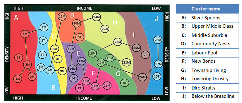
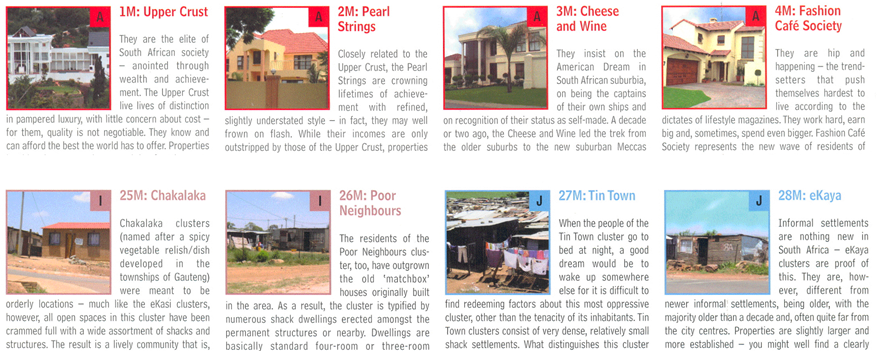
A few examples of the 38 classes in the typology are shown below, including four of the five classes in the Silver Spoons cluster, two of the three classes in the Dire Straits cluster and two of the three classes in the Below the Breadline cluster.
.
From the outset, the 38 classes of the settlement typology were used as development templates. The constructs of development templates and corresponding development template components allow UrbanSim to configure virtually any development proposal for construction in the future. The template structure is robust enough to cater for anything from a single house on an infill lot to a mixed use project with retail on the ground floor and apartments above.
While the development templates worked well, it proved exceptionally difficult to find suitable predictors of the market value of a property until the clusters were introduced as land-use typology. This was inspired by the observation that the cluster analysis done by the Knowledge Factory was based on factors which included household income, property value and dwelling type, so for residential properties at least one would expect to find a correlation between the newly defined land-use type and property value, which turned out to be true.
A potential disadvantage of using the clusters as a land-use typology was that it deviated from what municipal officials are used to. Fortunately UrbanSim allows for the definition of a number of typologies in addition to development templates and land use types. The plan type is one such typology that is used to define land use in the way that planners are accustomed to but in interactions with metros it seemed that most were indifferent to the definition of land use while one even welcomed it as a new way of thinking about their own data and processes.
Since the Knowledge Factory has replaced the Cluster Plus dataset with other products that are less useful for this specific purpose, the CSIR is investigating alternative means of deriving a suitable settlement typology.
In UrbanSim, households and jobs are located in specific buildings, which are in turn linked to specific cadastral parcels. The number of jobs that can be accommodated in a building depends on the floor space available in the building and the floor area required per job per sector of the economy. The total floor area is related to the total parcel area through the so-called ‘floor area ratio’. The number of households that can be accommodated on a parcel, which determines the density typically expressed as housing units per hectare also depends on the floor area per residential unit and the floor area ratio. The market value per residential unit may also depend on the floor area and parcel area.
Unlike the developed world where much of this information is available from municipal building records, we have to obtain the type of building from the ‘Building based land use type’ dataset of Geo Terra Image (GTI) and the rest from observed average densities per building/land use/development template type. This involves a fair amount of analysis for example to exclude outliers caused by building projects in progress from the calculations.
The GTI recently announced an enhanced product which includes building footprints and estimated number of storeys. This would be of great assistance, but is quite expensive and has not yet been acquired by the CSIR.
Information about business entities in South Africa is severely lacking and the best that we could do thus far is to create pseudo-buildings with sufficient floor space to accommodate the estimated number of jobs per economic sector but we cannot for example distinguish between businesses trading in clothing from businesses trading in fast foods, which prevents us from modelling agglomeration behaviours.
The trend in recent years for low-income households to prefer backyard shacks over informal settlements has had a profound effect on the morphology of our cities, with substantial changes in the density and resultant demand for services in some areas.
Based on its developed world origins, backyard shacks were probably not uppermost in the minds of the developers of the software. In the South African context it was essential to ensure that the phenomenon could be modelled. After investigation it was decided to define backyard shacks as a separate development template component and this eventually succeeded after various iterations of refinement and validation.
Given that in South Africa, 63% of households earn an income of less than R 2 408 per month (midpoint of income category from Census 2011), that 85% earn an income of less than R 9 591 per month and that a prolonged high unemployment ratio limits choice of work places, one could speculate that the value of time (spent commuting) would be different for lower income groups and that out-of-pocket expenses might be a stronger influencing factor than travel time for this (majority) segment of the population in South Africa.
This was approached by first undertaking a literature study to better understand the influence of commuting on the location choices made by households. The findings had a profound influence on the outcome of the work and on the functioning of the two most important models in UrbanSim, the Household Location Choice Model and Employment Location Choice Model. These models essentially produce spatial growth patterns to match demographic and economic control totals.
The question of whether commuting to work influences household location choices is a subset of a much wider body of knowledge on household behaviour and residential choice.
Many of these studies (regrettably mostly dated and undertaken in developed countries) have studied the determinants of intra-urban household relocation, often referred to as household (or residential) mobility. Some of these determinants include where a household (or individual) finds itself in the family life-cycle, type of tenure, income, education and of course place of work.
There seems to be widespread agreement that the family life cycle is one of the most important determinants of intra-urban mobility. This can result from families adjusting to changes in the family composition that accompany life cycle changes [Quigley and Weinberg 1977]. Stated another way, household mobility is primarily a response to a change in housing needs [Coulombel 2010 after Gobillon 2008].
The most obvious of these changes, household formation and household dissolution, are most likely to result in decisions to relocate. Changes in the head of the household, due to factors such as separation, divorce or death also increase the likelihood of relocation [Quigley and Weinberg 1977].
Single adults aged between 20 and 35 are by far the most mobile segment of the population where changes in personal, educational or employment domains are common triggers of relocation [Dieleman, Clark and Deurloo 2000].
The presence of school-going children in a family restricts mobility, with the incremental effect of additional children less than the first.
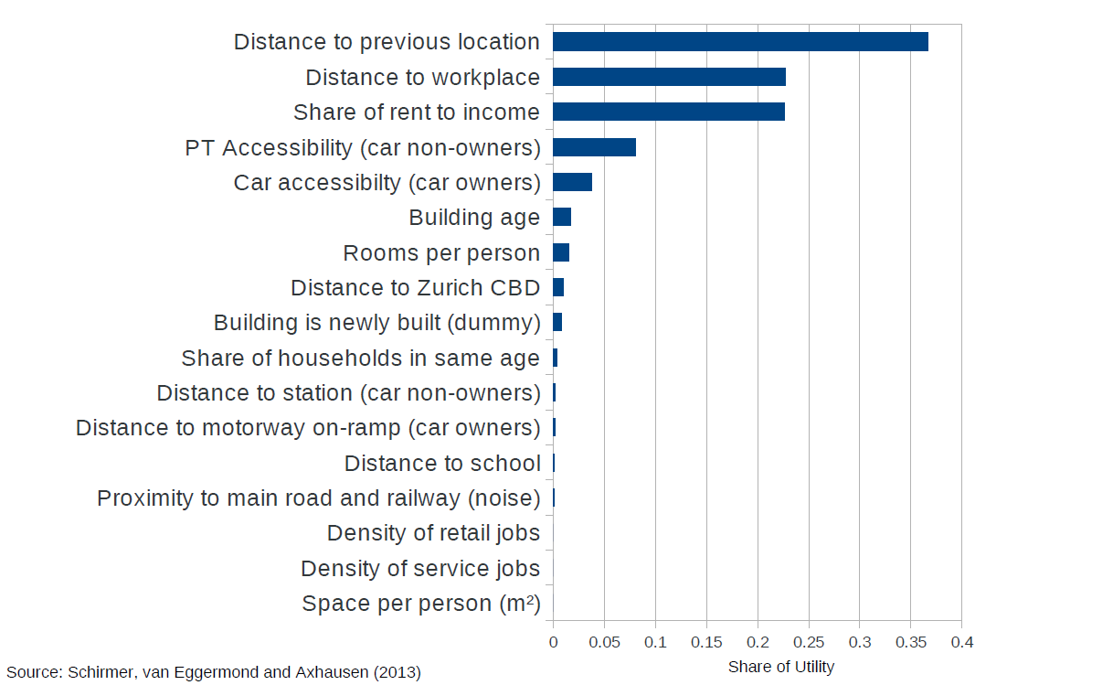
Another interesting finding is that moves by intact households often occur from origins within the same metropolitan area. This is supported by the latest UrbanSim model specification for Zürich, in which Renner, Schirmer and Müller [2013] found the distance from previous residence to be the most important predictor of household location choice (Figure 9).
Regarding type of tenure, there is persuasive evidence that renters are more likely to move than owners because the transaction costs associated with owning are substantially higher than those for renting. It also seems that prior mobility is strongly correlated with current mobility, which may in turn be influenced by the view that renting is cheaper than owning for those who move within 3 to 4 years of initial occupation [Quigley and Weinberg 1977]. It is estimated that two thirds of the population in Germany already do not own their own home [Goslett 2013] and there are some early indications that SA may follow trends in the developed world to favour renting over owning.
The influence of commuting on household mobility appears to be highly controversial [Coulombel 2010].
In urban economics (which would argue that relocation is an investment in the expectation of higher private returns) one would expect workplace location to exert significant influence on the decision to move (for example with increasing congestion or a job change). From an analysis of earlier empirical studies, Quigley and Weinberg [1977] found that “there is no consensus on the effects of accessibility, workplace location and workplace change on subsequent mobility” and that “accessibility and work-related reasons provide only minor impetus for residential mobility”. If cities were still predominantly mono-centric during that period one could explain the findings by noting that a job change would simply mean a change in location from one part of the CBD to another part of the CBD. If that simple, one would have expected the authors to comment, given that the “urban economics” of the time was very much based on the principle that the value/rent of land decreased with distance from the CBD or market place. The theory was later extended by adding household income classes and the notion of bid-rent (the maximum rent per surface unit that a household with given income is willing to pay at a specific location given a target utility [Fujita 1989].
To add to the controversy, other studies of the time found that a decrease in accessibility (measured in commute time or distance) increased mobility for both owners and renters [Quigley and Weinberg 1977].
In a more recent study undertaken under the auspices of EU-funded Sustain City project, Coulombel [2010] found residential choice (defined as “the choice of the place where the household lives, and, when it is dissatisfied with its current home, of when and where to move”) to be fairly complex. “A key issue when studying the link between employment location and residential mobility is that when facing costly commute (be it in time or money), two options arise: moving or quitting. The existence of a strong connection between the two processes is a well-established fact, theoretically and empirically (Zax 1994, Böheim and Taylor 1999, Gobillon 2001). The disagreement lies in the precise nature of this interaction. Böheim and Taylor (1999) are probably the most radicals in this regard, as they find commuting time to exert no significant influence on residential mobility. When Zax and Kain (1991) conclude that the longer the commute, the less likely moves are and the more likely quits are, implying that households would mainly resort to the “quit” strategy, Van Ommeren et al. (1999) find in the same case that moves and quits are both more likely. In the case of workplace relocation, Zax and Kain show the probability of a residential move to increase significantly with the distance between the new workplace and the old residence (Zax and Kain 1996). In short, this brief overview has, if anything, underlined the current lack of consensus over this topic, meaning that this case is not closed yet.”
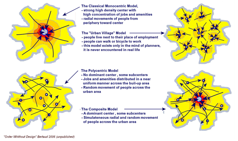
Though not mentioned in any of the articles referred to above, except by Coulombel [2010] in relation to mono-centric cities, the diagram below possibly provides an explanation to the discrepancies found in empirical studies on the influence of commuting on household mobility. The diagram is a conceptual illustration of the influence of city form (dispersal of land use) on trip patterns. As suggested before, a job change in a traditional monocentric city would simply mean a change in location from one part of the CBD to another part of the CBD, which would probably not warrant looking for another home. If the job change occurred in a poly-centric or composite city the result could be totally different. With cities being so different, a rigorous comparison of the influence of commuting on household mobility would require the cities in which the empirical studies were done to be classified by city form, something which would unfortunately be a study of on its own.
Up till now no attempt has been made to define commuting. One could think of various measures: Primarily mode, distance, time and cost, although many other factors such as convenience and personal safety presumably play a role in determining personal choice.
Most attempts at LUT modelling use travel time, distance or generalised cost as the most important descriptors of commuting. Generalized cost refers to the sum of the monetary and non-monetary costs of a trip. Monetary costs can in turn be split into fixed and variable costs. Fixed costs include vehicle finance (cost of capital), insurance, vehicle tracking and licenses. Running costs include fuel, maintenance (service and repair) and tyre wear. Non-monetary costs refer to the time spent undertaking the trip which can be converted to a monetary value by using a value of time, which varies according to the traveller's income and the purpose of the trip [Adapted from Wikipedia].
The use of distance as a descriptor of commuting probably stems from the fact that it is easy to determine and consistent with the reasoning process of real-world households that the model represents. Households do not consult transportation models when considering the location of a new house. For private vehicle trips they probably assume that practically all roads are congested during peak times and use distance as proxy for comparing the expected commute time from the new location to their current commute time.
The prevalence of travel time and generalised cost is understandable given the first world origins of the model and the value of time in these societies, but warrants further investigation in South Africa.
In South Africa the income distribution is significantly skewed towards lower incomes. It is well known that low income households have to spend proportionally more on transportation than higher income households and we have seen from our own work how the lowest income groups (typically found in informal settlements or backyard shacks) follow scarce job opportunities to minimize expenditure on transportation.
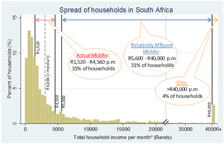
For the purpose of determining what percentage of households could be considered to belong to the ‘lower income groups’, various studies dealing with the definition of the ‘middle class’ were consulted [Visagie and Posel 2011][Visagie 2013] and the ‘lower income groups’ taken as all households with income less than the lower limit of the ‘middle class’. An example from Visagie [2013] is shown below based on the National Income Dynamics Study (NIDS) of 2008. While the actual breakpoints differ slightly from Census 2011 the overall conclusion was that about 65% of households with income less than about R 3 000 per month could be considered to have ‘low income’.
As such one could conclude that an UrbanSim model based on out-of-pocket expenses could be a more representative model for South Africa than one based on travel times and generalised cost.
Would such an approach sacrifice anything in terms of how the ‘Relatively Affluent’ and ‘Elite’ groups are accommodated in the model? To answer this question it must be pointed out that our implementation of UrbanSim deals with five income groups in different sub models of the Household Location Choice Model, allowing completely different variables to be used as predictors of behaviour for each income group. Only one variable, namely the generalised cost will not be available as a result of not having access to travel times. It should also be pointed out that it is no trivial matter to agree on the value of time and that even when travel times were available, they were rarely found to be more significant predictors of behaviours than distance-based variables. This has also been the finding from at least one of the case studies of the Sustain City project [Renner, Schirmer and Müller 2013], in which distance to workplace was found to be the second most important variable with ‘car accessibility’ (generalised cost) only the fifth most important (Figure 9).
One of the difficulties with the value of time is the difference between stated and revealed preferences of households. If one asked households belonging to the ‘Elite’ group it is likely that they would put a high value on time. Yet these same households may be found living in estates which are not centrally located and that would add to their daily travel time, indicating that they do not value time. The answer may simply be that there are other factors which are even more important, such as the aspirational value or safety and security considerations, which are often quoted as a reason for the popularity of various types of estates.
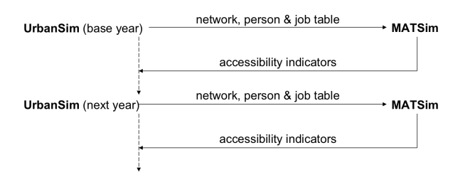
Because travel time and generalised cost depend on the congested state of the transportation network, they are usually obtained from a loose coupling between UrbanSim and a transportation model such as EMME, VISUM or lately MATSim (Figure 10). The ‘loose coupling’ is achieved by an exchange of data at the start of every UrbanSim simulation year as illustrated in the diagram on the next page [Nicolai and Nagel 2011]. Since this extends the total simulation time for a 30 year simulation period by many hours if not days for a study area such as the whole of Gauteng, the interactions are usually restricted to occur every 5 years or when there is a change in the network.
Another drawback of the traditional approach is that transportation models work with origin-destination (OD) pairs at a spatial resolution of Transportation Analysis Zones, which are coarse compared to the parcel geography used by UrbanSim. If MATSim is used to simulate individual travellers, it makes even less sense to base the loose coupling between UrbanSim and MATSim on travel time and generalised cost measures between OD pairs at such course geography. This is known to have caused peculiar zonal artefacts such as job opportunities in neighbouring zones being easier to reach than opportunities within the zone itself. The rate at which the size of OD matrices grow (by the square of the number of zones) rapidly limits increasing the spatial resolution by choosing smaller TAZs.
Due to the above constraints, others have started to look for alternatives [Nicolai and Nagel 2011] by exploring the notion of high resolution accessibility. The objective of this work was to determine if measures of accessibility based on pairs of locations could be replaced by measures based on attributes of the location itself, because this would significantly improve computational performance. The study was prompted by the observation that many of the variables used in specifications of the Household Location Choice Model all over the world appeared to be accessibility measures anyway, for example jobs within 30 min drive time, distance to workplace, etc. This agrees with our own experience and other papers from the EU-funded Sustain City project [Renner, Schirmer and Müller 2013].
Hansen [1959] defined accessibility as the potential of opportunities for interaction. If locations are otherwise equal, a location with easier access to activities like work, leisure or shopping is more attractive than locations with less access and have greater potential for residential development. Moeckel [2006] confirms that this approach is also true for businesses.
In high-resolution accessibility calculations, there are two resolutions to consider: One that determines for how many origins the accessibility is to be computed and another that determines to what level the destinations need to be resolved.
The number of origins was made variable in the form of squares measuring 250, 500, 1000, 2500, 5000, 7500 and 10000 meter per side. The number of destinations was taken as a 10% sample all job locations (more precisely the network nodes closest to the buildings with these jobs).
Nicolai and Nagel used a pre-existing UrbanSim/MATSim model of the Puget Sound Regional Council (which includes Seattle) to investigate the feasibility of calculating high resolution accessibilities for each of the seven origin square sizes.
The results demonstrated that it is computationally feasible to, for every origin; calculate a weighted sum over all possible destinations separately, rather than aggregating them into zones. This removes all zonal artefacts from the destination side of the computation. They also found that the spatial resolution of the origins had a strong impact, with resolutions smaller than 1000m x 1000m producing diminishing returns.
Although the previous section started out with a discussion of the onerous nature of coupling UrbanSim with transportation models, it should be noted that the study by Nicolai and Nagel was undertaken with the objective of improving the coupling rather than finding ways of avoiding it altogether. As long as generalised costs are used in the calculation of accessibility, the results will depend on the congested state of the network. In addition the results will also vary from one year to the next on account of where the jobs are located.
But what if out-of-pocket expenses can be used as an acceptable proxy for generalised costs in South Africa? In that case the cost and network distance-based measures of accessibility no longer depend on the congested state of the network and there is no need for coupling with transportation models, at least not for the purpose simulating urban growth. The remainder of this section explains how this possibility was investigated.
Note: If the scenarios to be simulated include indicators to assess their relative worth on the basis of changes in travel time, one would still have to run a transportation model, but this could be restricted to the start and end years of the simulation.
The investigation started by considering various software solutions to compute the lowest cost route (only the out-of-pocket component) between a potentially large number of origins and destinations. The routing algorithm was required to consider all modes of transport, including distance limited walking and cycling, private vehicles, unscheduled passenger vehicles and mass transit (bus and rail), as well as possible transfers between any of these modes.
After considering various alternatives, including ArcGIS Network Analyst, NetworkX and OpenTripPlanner it was decided to use OpenTripPlanner (OTP). The decision was based primarily on the following considerations:
Using OTP for the purpose envisaged here involves preparing XML configuration files and then running the JAVA code for OTP Graph Builder and OTP Batch Processor. The configuration files are required to set options and point the software to input and output folders. The Graph Builder converts an OSM file for the study area and a collection of General Transit Feed Specification (GTFS) files into a routable graph object required by the Batch Processor to determine the lowest cost route between any number of origins and destinations. The origins and destinations could be provided as GIS point or polygon features or as coordinates in a text file.
With OTP Analyst it is perfectly feasible to determine an accessibility indicator for every dissolved parcel even though this requires the lowest cost route over all modes of transport to be calculated from every dissolved parcel to every other dissolved parcel, a staggering number of calculations. This is made possible by the fact that OTP ‘remembers’ the result of previously considered routes to avoid unnecessary recalculation.
The term ‘dissolved parcel’ refers to the merging of adjacent cadastral parcels of the same development template into a contiguous area typically limited to a street block in built-up areas. Mindful of the conclusion reached by Nicolai and Nagel [2010] that nothing is gained by using origins smaller than about 1 km2, dissolved parcel-based origins (typically 20 to 50 times smaller) do seem wasteful, even though the calculations only have to be repeated when the network changes. It was therefore decided to rather use ‘modified small areas’ as origin and destination zones. These were derived from the STATSSA small area geography by retaining the small areas (with median area of about 0.1 km2 in NMBM) in fully built-up areas and subdividing the larger areas so that parcels have a maximum area of about 2.5 km2.
Regarding the destinations, it would likewise be feasible to use the dissolved parcels were jobs are located because the centroid of a street block would present a very similar routing request to OTP than the ‘nearest network node to buildings with jobs’ Nicolai and Nagel [2010].
The only problem with this approach, as mentioned before, is that the locations of jobs change from one simulation year to the next. If this required OTP to run every year it would not really represent progress from the perspective of avoiding coupling to transportation models.
To avoid this it was decided to store the results of the lowest-cost routing for different modes per OD pair. This allows weighted measure of accessibility to be calculated as UrbanSim variables using the job locations for the correct simulation year. It also opens up numerous other possibilities to customise accessibility for jobs in different sectors of the economy, for households of different income groups, etc. All this can be achieved by using standard UrbanSim functionality to define new variables.
This solution flies in the face of the efforts of Nicolai and Nagel [2010] to get rid of storing OD pairs, but is well worth it if it avoids repeatedly running OTP or MATSim. For example, in Nelson Mandela Bay with 2672 modified small areas, the OD matrix has 7.14 million rows and 6 columns, taking up 512 MB of storage. The Graph Builder runs in less than a minute, while the Batch Processor and subsequent R scripts developed to piece together separate output files for each origin completes within 30 minutes on an ordinary laptop computer. As mentioned before it only has to be repeated when a different scenario requires the network to change. If the change is to the road network, the changes will be introduced as a modified OSM file for the scenario in question. If the change involves transit developments such as the introduction of a BRT or extension of Gautrain routes, the new routes and stops simply have to be added to the GTFS files.
If the OD matrix becomes a constraint for large study areas, there is the option to cut the size in half by changing it to a symmetrical matrix on account of the fact that the cost of a trip from A to B will only differ marginally from the trip from B to A. For now it does not pose a limitation at all.
Selected results obtained from OTP Analyst using Nelson Mandela Bay as case study are provided in this section, based on the following inputs:
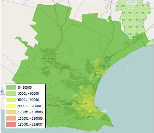
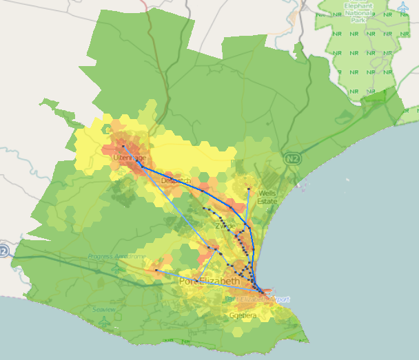
Based on the above inputs the numbers of non-home-based jobs that can be reached from an origin zone by different modes of transport for an out-of-pocket expense of less than R40 per return trip are shown in Figure 11 and Figure 12.
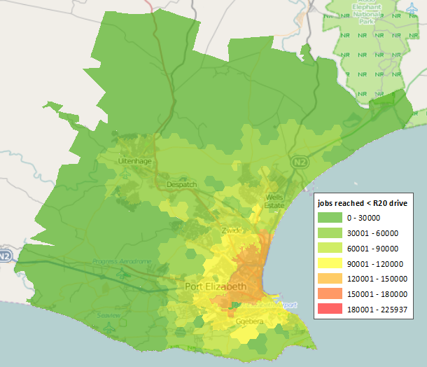
The threshold of R40 per day was chosen somewhat arbitrarily as close to 25% of the R 3 000 upper limit of the ‘low income’ group. Only non-home-based jobs are considered because home-based jobs per definition do not involve travelling to work. The mode described as ‘drive-alone’ represents a trip by single occupancy vehicle at a rate of R1.48 per km with no part of the trip being transit. This is considered to be the mode of choice of the ‘Elite’ group (Figure 8). The mode described as ‘transit’ represents a trip by rail if available, otherwise by BRT if available or failing that by minibus taxi at a rate of R1.14 per km. This is considered to be the mode of choice for the ‘low income’ group of households.
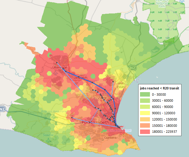
The previous two maps confirm a dramatic increase in the number of jobs that can potentially be accessed by transit for under R40 per day. For the drive-alone mode there are no zones that can even access the 150 000 jobs category (59% of the 253 803 non-home-based jobs in 2001) but for the transit mode, a large number of zones are able to access the top category of 180 000 jobs (71%) and the most accessible zone is able to access 89% of all the non-home-based jobs available in the city for under R40 per day!
By comparison of Figure 11 and Figure 12 one could venture to say that in terms of urban form (Figure 7), transit holds the potential of changing NMBM from a monocentric to a polycentric city.
Even if the threshold is reduced to R20 per return trip, Figure 13 below (with same legend as before) tells the same story, some zones able to access more than 150 000 jobs.
For more information contact:
Quinton van Heerden, CSIR
qvheerden@csir.co.za